Importing Library
import matplotlib.pyplot as plt       #Creating Plots
import numpy as np                    #Working with numeric array
import random
import time
Misc
%matplotlib notebook                  #Makes Notebook zoom-able & resize-able
random.seed(61)                       #Generate same random numbers on multiple executions
Generating Dataset
x_data = np.array([-7.5,-2.5,4,9])    #Input data
y_data = np.array([-1.5,2.5,4.5,7])   #Output data
Defining model
def run_model(x):
  global m,c                          #Making Variable Global for Simplicity
  y = m*x + c                         #Predicting value(Output)
  return y                            #Returning prediction
Define intial Value of parametrs
m = random.uniform(-1,1)              #Random slope, Dosen't really matter
c = random.uniform(-10,-5)            #Random intercept
Makeing intial prediction
y_init = run_model(x_data) #Prediction with randomly Generated m and c
Plotting Intial Model and Data
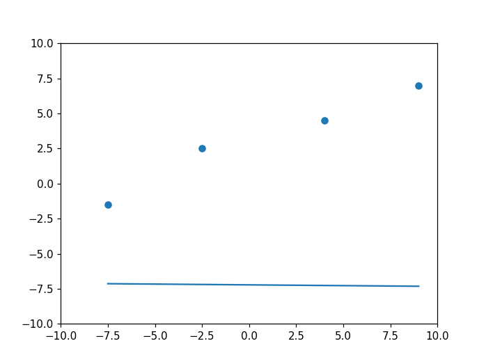
fig = plt.figure()                    #Create a new figure
plt.axis([-10, 10, -10, 10])          #Size of plot
plt.scatter(x_data,y_data)            #Plotting data
plt.plot(x_data,y_init)               #Plotting model
fig.canvas.draw()                     #Rendering plot
Defining Learn Rate and iterations/epochs
learn_rate = 0.01                     #Rate of learning
iterations = 100                      #Number of Epochs
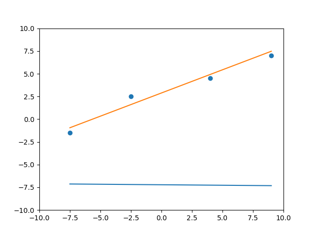
Training Model
for i in range(iterations):           #Loop to iterate
  for x,t in zip(x_data,y_data):      #Loop through data
      y = run_model(x)                #Making prediction
      error = np.abs(t - y)           #Error in prediction, Absolute difference of prediction and true value
      m = m + learn_rate*error*x      #Updating slope
      c = c + learn_rate*error        #Updating intercept
      time.sleep(0.1)                 #Slowing down training, You can comment this out

  y_next = run_model(x_data)          #Prediction on Updated Model for Plotting

  line, = plt.plot(x_data,y_next)     #Plotting new model
  fig.canvas.draw()                   #Rendering plot
  line.remove()                       #Removing Model
Plotting Final Model
plt.plot(x_data,y_next)               #Plotting final model
fig.canvas.draw()                     #Rendering plot
print(error,m,c)                      #Printing model parameters(slope and intercept)
Using scikit-learn library
Importing Library
from sklearn import linear_model
Generating and reshaping Dataset
x_data = np.array([-7.5,-2.5,4,9]).reshape([-1, 1])
y_data = np.array([-1.5,2.5,4.5,7]).reshape([-1, 1])
Loading Model
regr = linear_model.LinearRegression()
Training
regr.fit(x_data,y_data)
Making prediction
y_pred = regr.predict(x_data)
Plotting
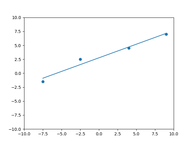
fig = plt.figure()
plt.axis([-10, 10, -10, 10])
plt.scatter(x_data,y_data)
plt.plot(x_data,y_pred)
fig.canvas.draw()